Subsections

• The rate constants for adenylate kinase
• NAD/NADH concentrations
• The rate constants for haemoglobin
• Calcium dynamics
• NO dynamics
• Myosin phosphorylation and dephosphorylation
• Electron transport

Particular calculations: biochemistry

The rate constants for adenylate kinase

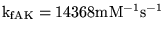
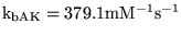
We use the rate constants given in (5) to calculate effective rate constants for adenylate kinase. We need effective rate constants because the actual reactants may be free or magnesium bound.

We have from (5) the rate for the reaction as:

$$\ensuremath{\mathrm{k_{fAK}[ADP_f][ADP_{Mg}] - k_{bAK}[ATP_{Mg}][AMP]}}$$ (55)

where $\ensuremath{\mathrm{[ADP_f]}}$ and $\ensuremath{\mathrm{[ADP_{Mg}]}}$ are free and magnesium bound versions of ADP and the same goes for ATP. In our units, $\ensuremath{\mathrm{k_{fAK}}}= 14368 \ensuremath{\mathrm{mM^{-1}s^{-1}}}$ and $\ensuremath{\mathrm{k_{bAK}}}= 379.1 \ensuremath{\mathrm{mM^{-1}s^{-1}}}$. Also, $\ensuremath{\mathrm{[ADP_f]}}\simeq 0.0798\ensuremath{\mathrm{[ADP_{tot}]}}$, $\ensuremath{\mathrm{[ADP_{Mg}]}}\simeq 0.92\ensuremath{\mathrm{[ADP_{tot}]}}$, $\ensuremath{\mathrm{[ATP_{Mg}]}}\simeq \ensuremath{\mathrm{[ATP_{tot}]}}$. So, if we assume that the concentration of magnesium doesn't change, we can write the rate equation:

$$\ensuremath{\mathrm{k_{ADPATP}[ADP_{tot}]^2 - k_{nADPATP}[ATP_{tot}][AMP]}}$$ (56)

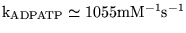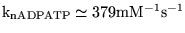we get that $\ensuremath{\mathrm{k_{ADPATP}}}\simeq 1055 \ensuremath{\mathrm{mM^{-1}s^{-1}}}$ and $\ensuremath{\mathrm{k_{nADPATP}}}\simeq 379 \ensuremath{\mathrm{mM^{-1}s^{-1}}}$. These are the values that we use. We also have for the effective equilibrium constant: $\ensuremath{\mathrm{Keq_{ADPATP}}}\equiv \ensuremath{\mathrm{k_{ADPATP}}}/\ensuremath{\mathrm{nk_{ADPATP}}}\simeq 2.78$.

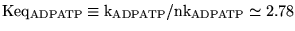NAD/NADH concentrations

We have that the average NAD concentration in a cell is:

$$\frac{\ensuremath{\mathrm{[NAD_{cyt}]}}Vol_{cyt} + \ensuremath{\mathrm{[NAD_{im}]}}Vol_{im}}{Vol_{cyt} + Vol_{im}}$$ (57)

In (6) it is stated from work done on the rat heart that the mitochondria possess 72 per cent of cellular NAD content, i.e.

$$0.28\ensuremath{\mathrm{[NAD_{im}]}}Vol_{im} = 0.72\ensuremath{\mathrm{[NAD_{cyt}]}}Vol_{cyt}$$ (58)

Assuming that we know the relative volumes of cytoplasm and mitochondria, and also know the average concentration of NAD in a cell (given in for example (7)) we can calculate the cytoplasmic and mitochondrial concentrations from these two equations.

The rate constants for haemoglobin

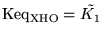
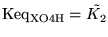
In this section we are interested in the equilibria of the four chemical reactions involving haemoglobin, oxygen and protons. Two equilibrium constants - $\ensuremath{\mathrm{Keq_{XH}}}$, $\ensuremath{\mathrm{Keq_{XO4H}}}$ - can be found in the literature, leaving $\ensuremath{\mathrm{Keq_{XHO}}}$ and $\ensuremath{\mathrm{Keq_{XO4}}}$ to be determined. We first note that although $\ensuremath{\mathrm{Keq_{XH}}}$, $\ensuremath{\mathrm{Keq_{XO4H}}}$ are defined as usual in the literature, the last two - $\ensuremath{\mathrm{Keq_{XHO}}}$ and $\ensuremath{\mathrm{Keq_{XO4}}}$ - we define somewhat differents. For completeness we state all the definitions:

$$\ensuremath{\mathrm{Keq_{XH}}}= \frac{\ensuremath{\mathrm{[H... ...th{\mathrm{[Hb(H^+)_{n_H}]}}\ensuremath{\mathrm{[O_2]^{2.5}}}}$$ (59)

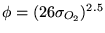
because we treat the combination of haemoglobin with oxygen as a generalised reaction whose rate is proportion to the $\ensuremath{\mathrm{[O_2]^{2.5}}}$. It is more convenient to use these definitions rather than the usual definitions based on the stoichiometry. Despite this difference, some basic algebra (as in (3), Section 16.2) tells us that:

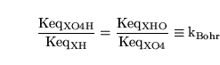$$\frac{\ensuremath{\mathrm{Keq_{XO4H}}}}{\ensuremath{\mathrm{... ...math{\mathrm{Keq_{XO4}}}} \equiv \ensuremath{\mathrm{k_{Bohr}}}$$ (60)

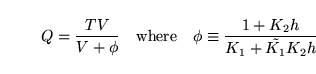
where this equation defines $\ensuremath{\mathrm{k_{Bohr}}}$. We now come to the rather tricky question of where to get another equation allowing the determination of all the equilibria.

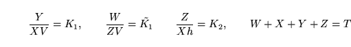
We follow (3), Section 16.2. To simplify notation we define $\ensuremath{\mathrm{[Hb(O_2)_4]}}= Y$, $\ensuremath{\mathrm{[Hb]}}= X$, $\ensuremath{\mathrm{[Hb(O_2)_4(H^+)_{n_H}]}}= W$, $\ensuremath{\mathrm{[Hb(H^+)_{n_H}]}}= Z$, $\ensuremath{\mathrm{[H^+]}}= h$, $\ensuremath{\mathrm{[O_2]^{2.5}}}= V$, $\ensuremath{\mathrm{Keq_{XO4}}}= K_1$, $\ensuremath{\mathrm{Keq_{XHO}}}= \tilde{K_1}$, $\ensuremath{\mathrm{Keq_{XH}}}= K_2$, $\ensuremath{\mathrm{Keq_{XO4H}}}= \tilde{K_2}$ and $T =$ the total haemoglobin in all forms. In this notation, at equilibrium we have the following four equations for the combination of haemoglobin with oxygen and protons:

$$\frac{Y}{XV} = K_1, \qquad \frac{W}{ZV} = \tilde{K_1} \qquad \frac{Z}{Xh} = K_2, \qquad W + X + Y + Z = T$$ (61)

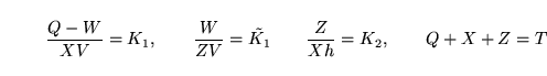
To obtain a fourth equation we will do the following: First we need to obtain a function describing the total oxygen saturation $(Y+W)/T$ as a function of oxygen tension. Then we can compare this function to empirically obtained functions to set our fourth rate constant. This all takes some algebra.

We rewrite the equations in terms of the variable $Q \equiv Y + W$, eliminating $Y$ to get:

$$\frac{Q-W}{XV} = K_1, \qquad \frac{W}{ZV} = \tilde{K_1} \qquad \frac{Z}{Xh} = K_2, \qquad Q + X + Z = T$$ (62)

We substitute for $X$ into the last of these to get:

$$Q + Z\left(1 + \frac{1}{K_2 h}\right) = T$$ (63)

We solve the first and third equations for $X$ to get:

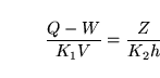$$\frac{Q-W}{K_1 V} = \frac{Z}{K_2 h}$$ (64)

and solve this for $W$:

$$W = Q - \frac{ZK_1 V}{K_2 h}$$ (65)

We combine this with the second equation for $W$ ( $W = \tilde{K_1}ZV$) to get:

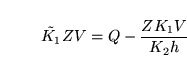$$\tilde{K_1}ZV = Q - \frac{ZK_1 V}{K_2 h}$$ (66)

and rearrange to get:

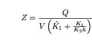$$Z = \frac{Q}{V\left(\tilde{K_1} + \frac{K_1}{K_2 h}\right)}$$ (67)

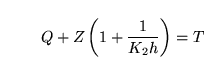
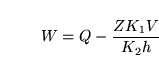
Finally we substitute back for $Z$ into 63 to get:

$$Q\left(1 + \frac{1 + \frac{1}{K_2 h}}{V\left(\tilde{K_1} + \frac{K_1}{K_2 h}\right)}\right) = T$$ (68)

This can be rearranged to give:

$$Q = \frac{T V}{V + \phi} \quad \mbox{where} \quad \phi \equiv \frac{1 + K_2 h}{K_1 + \tilde{K_1}K_2 h}$$ (69)

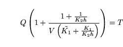
This equation is important because it is known from empirical investigations of the dissociation curve for haemoglobin at pH 7.4 that half-maximal saturation occurs at oxygen partial pressures of about 26 mmHg. In other words at pH 7.4 the curve:

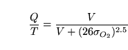$$\frac{Q}{T} = \frac{V}{V + (26 \sigma_{O_2})^{2.5}}$$ (70)

where $\sigma_{O_2}$ is the solubility of oxygen in blood, reproduces the dissociation curve well. We can use this estimate for $\phi$ to calculate the final equilibrium constant. Substituting $\ensuremath{\mathrm{k_{Bohr}}}= \frac{\tilde{K_1}}{K_1} = \frac{\tilde{K_2}}{K_2}$ gives:

$$\phi = \frac{1}{K_1}\left(\frac{1 + K_2 h}{1 + \ensuremath{\mathrm{k_{Bohr}}}K_2 h}\right)$$ (71)

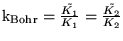
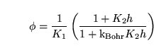
Setting $\phi = (26 \sigma_{O_2})^{2.5}$, putting the value for $h$ at pH 7.4, and rearranging gives:

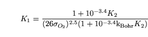$$K_1 = \frac{1 + 10^{-3.4}K_2 }{(26 \sigma_{O_2})^{2.5}(1 + 10^{-3.4}\ensuremath{\mathrm{k_{Bohr}}}K_2 )}$$ (72)

Or in terms of the original variables:

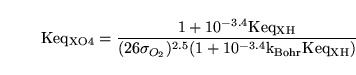$$\ensuremath{\mathrm{Keq_{XO4}}}= \frac{1 + 10^{-3.4}\ensurem... ...\ensuremath{\mathrm{k_{Bohr}}}\ensuremath{\mathrm{Keq_{XH}}})}$$ (73)

Thus equations 60 and 73 can be used to determine $\ensuremath{\mathrm{Keq_{XHO}}}$ and $\ensuremath{\mathrm{Keq_{XO4}}}$.

Finally we mention that the actual rate constants (as opposed to these equilibrium constants) are then calculated using the methodology in section 2.2.1 from equilibrium and half-time data.

Calcium dynamics

Calcium is assumed to be supplied by a process dependent on the membrane potential, and removed by an active mechanism. The total dynamics for calcium are:

$$\ensuremath{\mathrm{\dot{[Ca_{i, j}^{2+}]} = k_{Cain, j} - \... ...t} + \ensuremath{\mathrm{[Ca_{i, j}^{2+}]}}}}}\quad\quad j=1,2$$ (74)

At steady state we therefore have in segment j :

$$\ensuremath{\mathrm{[Ca_{i, j}^{2+}]_n = \frac{k_{Cain, j, n}Km_{Caout}}{Vmax_{Caout, j} - k_{Cain, j, n}}}}\quad\quad j=1,2$$ (75)

Linearising about this steady state value gives us to first order:

$$\dot \delta_j = -\frac{\ensuremath{\mathrm{Vmax_{Caout, j}}}... ...math{\mathrm{Km_{Caout} [Ca_{i, j}^{2+}]_n}}} \quad\quad j=1,2$$ (76)

where $\delta_j$ is a small perturbation to $\ensuremath{\mathrm{[Ca_{i, j}^{2+}]}}$. From this we derive the relation:

$$t_{1/2, \ensuremath{\mathrm{Ca}}} = \ensuremath{\mathrm{\fra... ...out} + [Ca_{i, j}^{2+}]_n)}{Vmax_{Caout, j}}}}\quad\quad j=1,2$$ (77)

Here $t_{1/2, \ensuremath{\mathrm{Ca}}}$ is an approximate half-time for Calcium inflow and outflow which we assume to be the same in each segment. We assume that we can find $t_{1/2, \ensuremath{\mathrm{Ca}}}$, $\ensuremath{\mathrm{[Ca_{i, j}^{2+}]_n}}$ and $\ensuremath{\mathrm{Km_{Caout}}}$ in the literature and equations 75 and 77 to determine $\ensuremath{\mathrm{k_{Cain, j, n}}}$ and $\ensuremath{\mathrm{Vmax_{Caout, j}}}$. We define a parameter $\ensuremath{\mathrm{Km_{Caout, ratio} = Km_{Caout}/[Ca_{i, 1, n}]}}$, and note that if $\ensuremath{\mathrm{Km_{Caout, ratio}}}$ is small this implies that the cells' ability to extrude calcium is rapidly reached.

NO dynamics

The dynamics for NO are very simple:

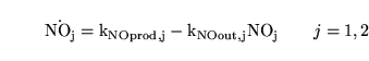$$\dot{\ensuremath{\mathrm{NO_j}}} = \ensuremath{\mathrm{k_{NO... ...}}}- \ensuremath{\mathrm{k_{NOout, j}NO_j}}\quad\quad j = 1, 2$$ (78)

At equilibrium we expect:

$$\ensuremath{\mathrm{[NO_j]_n = \frac{k_{NOprod, j, n}}{k_{NOout, j}}}}\quad\quad j = 1, 2$$ (79)

By linearising equation 78 we obtain the expression for the halftime:

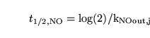$$t_{1/2, \ensuremath{\mathrm{NO}}} = \ensuremath{\mathrm{\log(2)/k_{NOout, j}}}$$ (80)

As with calcium, we currently assume that the halftime is the same in both segments. We treat $\ensuremath{\mathrm{[NO_j]_n}}$ and $t_{1/2, \ensuremath{\mathrm{NO}}}$ as parameters to be determined from the literature, and use them to determine $\ensuremath{\mathrm{k_{NOprod, j, n}}}$ and $\ensuremath{\mathrm{k_{NOout, j}}}$ using equations 79 and 80.

Myosin phosphorylation and dephosphorylation

We assume that the total quantity of myosin in the cell remains constant at some value $\ensuremath{\mathrm{MLC_{tot}}}$, i.e.

$$\ensuremath{\mathrm{MLC_{tot}}}\equiv \ensuremath{\mathrm{[MLC_{p, j}]}}+ \ensuremath{\mathrm{[MLC_j]}}$$ (81)

which we currently assume to be the same in each section. We also define a parameter describing the normal fraction of unphosphorylated myosin heads in each segment:

$$\ensuremath{\mathrm{MLC_{frac, j} \equiv [MLC_j]_n/MLC_{tot}}}\quad\quad j = 1,2$$ (82)

We then treat $\ensuremath{\mathrm{MLC_{tot}}}$ and $\ensuremath{\mathrm{MLC_{frac, j}}}$ as parameters to be determined from the literature and use equations 81 and 82 to determine $\ensuremath{\mathrm{[MLC_j]_n}}$ and $\ensuremath{\mathrm{[MLCp_j]_n}}$.

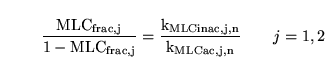
At equilibrium we have:

$$\frac{\ensuremath{\mathrm{[MLC_{p, j}]_n}}}{\ensuremath{\mat... ...\frac{k_{MLCac, j, n}}{k_{MLCinac, j, n}}}}\quad\quad j = 1,2$$ (83)

From this equation we get that:

$$\ensuremath{\mathrm{\frac{[MLC_j]_n}{MLC_{tot} - [MLC_j]_n} = \frac{k_{MLCinac, j, n}}{k_{MLCac, j, n}}}}\quad\quad j = 1,2$$ (84)

i.e.

$$\ensuremath{\mathrm{\frac{MLC_{frac, j}}{1 - MLC_{frac, j}} = \frac{k_{MLCinac, j, n}}{k_{MLCac, j, n}}}}\quad\quad j = 1,2$$ (85)

A linearisation about the fixed point now gives:

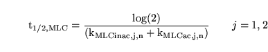$$\ensuremath{\mathrm{t_{1/2, MLC}}}= \frac{\log(2)}{\ensurema... ...rm{(k_{MLCinac, j, n} + k_{MLCac, j, n})}}} \quad\quad j = 1,2$$ (86)

We now treat $\ensuremath{\mathrm{t_{1/2, MLC}}}$ as a parameter to be determined from the literature, and use equations 85 and 86 to determine $\ensuremath{\mathrm{k_{MLCinac, j, n}}}$ and $\ensuremath{\mathrm{k_{MLCac, j, n}}}$.

Electron transport

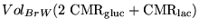In section 3 above, we noted that the gross production of $\ensuremath{\mathrm{NADH}}$ and $\ensuremath{\mathrm{FADH_2}}$ are equal to $Vol_{BrW}(10 \ensuremath{\mathrm{CMR_{gluc}}}+ 5 \ensuremath{\mathrm{CMR_{lac}}})$ and $Vol_{BrW}(2 \ensuremath{\mathrm{CMR_{gluc}}}+ \ensuremath{\mathrm{CMR_{lac}}})$ respectively. We also noted that this implies that $\ensuremath{\mathrm{CMRO_2}}= 6 \ensuremath{\mathrm{CMR_{gluc}}}+ 3 \ensuremath{\mathrm{CMR_{lac}}}$.

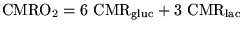We can use these data to calculate $\ensuremath{\mathrm{Vmax_{NQ}}}$ and $\ensuremath{\mathrm{Vmax_{FQ}}}$. Let $\ensuremath{\mathrm{T_{NQ}}}$ be the turnover rate for oxygen in the equation for the oxidation of $\ensuremath{\mathrm{NADH}}$, and $\ensuremath{\mathrm{T_{FQ}}}$ be the turnover rate for oxygen in the equation for the oxidation of $\ensuremath{\mathrm{FADH_2}}$. Then we get the equations:

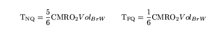$$\ensuremath{\mathrm{T_{NQ}}}= \frac{5}{6}\ensuremath{\mathrm... ...hrm{T_{FQ}}}= \frac{1}{6}\ensuremath{\mathrm{CMRO_2}}Vol_{BrW}$$ (87)

which can be solved for $\ensuremath{\mathrm{Vmax_{NQ}}}$ and $\ensuremath{\mathrm{Vmax_{FQ}}}$.