


Next: Metabolic rates and accounting
Up: All model parameters
Previous: Basics
Subsections
Estimating rate constants for reactions
We now describe some methodologies that we use frequently for estimating rate constants in reactions.
Estimating rate constants from equilibrium and turnover data for reactions not normally at equilibrium
Consider a generalised reaction of the form:
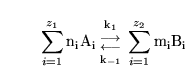 |
(6) |
with, for maximum generality, substrate
 residing in a compartment with volume
  and product
 residing in a compartment with volume
  .
Let
.
Let
![$a_i \equiv [A_i]$](img40.png) , etc. What we mean by the above representation is that we have the dynamics:
, etc. What we mean by the above representation is that we have the dynamics:
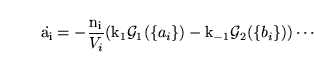 |
(7) |
etc. for some functions  and
and  .
.
 and
and
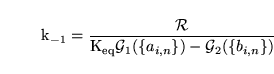
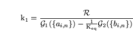
 could represent either mass action rates, or Vmax values if the reaction actually consists of two opposing saturable processes. Quantities we might have access to are the normal turnover rate:
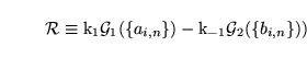 |
(8) |
and the ratio
 (calculable from the equilibrium concentrations of the reactants and products if it is a mass-action reaction). Then we can calculate:
 |
(9) |
and similarly:
 |
(10) |
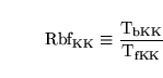
Alternatively we might have an estimate for the normal ratio of backward to forward reaction rates (i.e. of the degree of bi-directionality of the reaction at normal substrate concentrations). In such cases we often define a quantity:
 |
(11) |
In some situations - for example in the conversion of lactate to pyruvate in the brain - we know that a reaction is near equilibrium in normal conditions, but cannot actually be at equilibrium. We can use such heuristic knowledge by setting the value of
 to be near one.
As an example of the application of these methods, consider the transport of potassium ions across the blood brain barrier. This processes is known to be active, bi-directional, and possibly involving multiple mechanisms (2) . To avoid extensive complications, in the current version of the model we describe the sum of these processes very simply via two Michaelis Menten reactions:
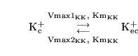 |
(12) |
Further we assume for simplicity the same Km value in each direction. (i.e. a single kind transporter, but perhaps expressed in different quantities on each side of the barrier). We now calculate the forward and backward Vmax values for the transport of potassium from blood to brain, i.e.
 and
and
 . Let
. Let
 and
and
 be the normal forward and backward transport rates, i.e.
![\begin{displaymath}
\ensuremath{\mathrm{T_{fKK}}}= \ensuremath{\mathrm{Vmax1_{KK...
...ax2_{KK}}}\ensuremath{\mathrm{[K^+_{ec}]/(Km_{KK} + K^+_{ec})}}\end{displaymath}](img55.png) |
(13) |
We must have that at steady state the difference between these rates is the same as the rate of transport of potassium out of the extracellular space during CSF drainage:
![\begin{displaymath}
\ensuremath{\mathrm{T_{fKK}}}- \ensuremath{\mathrm{T_{bKK}}}= \ensuremath{\mathrm{[K^+_{ec}]}}G_o(P_{ic} - P_{vs})
\end{displaymath}](img56.png) |
(14) |
where  is a parameter representing the conductance to CSF outflow,
  is intracranial pressure, and
  is venous pressure. If we can estimate:
 |
(15) |
then we can calculate that
![\begin{displaymath}
\ensuremath{\mathrm{T_{fKK}}}= \frac{\ensuremath{\mathrm{[K^...
...]}}G_o(P_{ic} - P_{vs})}{(1 - \ensuremath{\mathrm{Rbf_{KK}}})}
\end{displaymath}](img61.png) |
(16) |
from which we calculate
and
.
This methodology is used very frequently in the biochemical part of the model because as we shall see in section 3 we quite often can calculate reasonable estimates of the normal flux through a particular reaction pathway.
We note a fact that we use often in estimating parameters for the model: This is that reliable and reproducible estimates of maximum rates of reaction (or alternatively of enzyme concentrations and specific activities) are hard to come by for the human brain in vivo. Because we are much more likely to have reasonable estimates of the normal flux through a reaction, and because other constants such as Km values can be more reliably estimated from in vitro experimental data, we almost never use experimental Vmax values, even where they are available, and instead using the techniques above to estimate them.
Estimating rate constants for reactions from equilibrium, concentration and half-time data
One compartment
Sometimes we are ignorant about the normal flux through a reaction pathway. Alternatively, sometimes the very structure of a model implies that at model steady state, a reaction must be at equilibrium, i.e. the flux must be zero. For example, given a reaction  with reactants
, if for any one of the reactants, is the only reaction in which it partakes, then at steady state (if the model achieves a steady state!) must be at equilibrium.
with reactants
, if for any one of the reactants, is the only reaction in which it partakes, then at steady state (if the model achieves a steady state!) must be at equilibrium.
In both of these situations, we might have knowledge of the equilibrium constant but this is not sufficient to determine the actual values of the reaction rates. For this we need further information. The quantity that we most frequently use to determine the rate constants in such situations is a putative half-time to reach equilibrium for the reaction.
To make this concept more precise, consider a generalised reaction:
|
(17) |
For the time being we assume that all reactants and products are in one compartment, though sketch the (simple) generalisation at the end. Let
 ,
,
 , and again
, etc. Considered as a dynamical system, evolution is in the
, and again
, etc. Considered as a dynamical system, evolution is in the  -dimensional space of chemical concentrations. We are of course only interested in the area where all
  . We call this quadrant
  , and a given point in it
  . The equilibria of this reaction form a co-dimension 1 surface in this space
 , defined as the set of points satisfying the equation:
 |
(18) |
Any disturbance away from the surface of equilibria relaxes to a unique point on  .
.
We get the dynamics:
 |
(19) |
Because
 for all
  and similarly
 for all
 , given an initial condition we can determine the unique path by which an initial point
 relaxes to the final point
 . This is done simply by integrating the above relations to get:
 |
(20) |
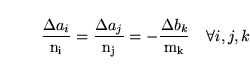
where
 , etc. Given an initial condition
  , the above equations define the line in along which the system evolves to reach a point on . The point on reached is derived by considering in addition equation 18.
This geometry means that there is a unique eigenvalue associated with any given point on the surface and hence any given initial condition.
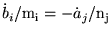
Perturbing equations 19 by letting
 and
and
 , we get the linearised equations:
That the same equation holds for all  and
and  is not surprising considering the topology of the system which requires that any perturbation which is to approach a particular equilibrium solution must do so along a particular path.
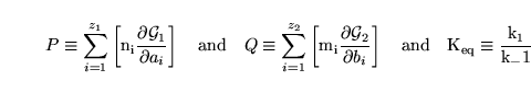
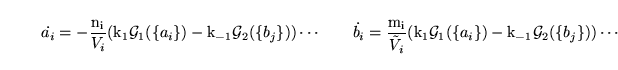
We can work out the halftime for relaxation to equilibrium to be:
![\begin{displaymath}
t_{1/2} = \frac{\ln 2}{\left(\ensuremath{\mathrm{k_1}}\sum_{...
...\mathrm{m_i}}\frac{\partial \mathcal{G}_2}{b_i}\right]\right)}
\end{displaymath}](img90.png) |
(22) |
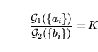
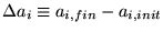
Let:
 |
(23) |
Note that this definition of
 is not equivalent to the usual definition of the equilibrium constant unless the dynamics are mass action, but is more convenient for our purposes. So we get:
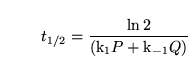 |
(24) |
We can then solve for
and
in terms of  and
, i.e.
and
, i.e.
 |
(25) |
Thus if we know
and have an estimate for at given equilibrium concentrations of reactants, then we can calculate estimates of
and
.
Take the particular case of a mass action reaction. In this case
 and
and
 . So that:
![\begin{displaymath}
\ensuremath{\mathrm{n_i}}\frac{\partial \mathcal{G}_1}{\part...
...od_{j=1, j\not= i}^{z_2}b_j^{\ensuremath{\mathrm{m_j}}}\right]
\end{displaymath}](img98.png) |
(26) |
giving:
![\begin{displaymath}
P \equiv \sum_{i=1}^{z_1}\left[\ensuremath{\mathrm{n_i}}^2 a...
...od_{j=1, j\not= i}^{z_2}b_j^{\ensuremath{\mathrm{m_j}}}\right]
\end{displaymath}](img99.png) |
(27) |
As a somewhat non-trivial example we consider the generalised reaction:
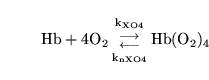 |
(28) |
with the forward rate of reaction depending on
![$\ensuremath{\mathrm{[O_2]^{2.5}}}$](img101.png) . i.e.:
. i.e.:
![\begin{displaymath}
\dot{\ensuremath{\mathrm{Hb}}} = - \ensuremath{\mathrm{k_{XO...
...\ensuremath{\mathrm{k_{nXO4}}}\ensuremath{\mathrm{[Hb(O_2)_4]}}\end{displaymath}](img102.png) |
(29) |
In this case:
![\begin{displaymath}
\mathcal{G}_1 = \ensuremath{\mathrm{[Hb][O_2]^{2.5}}}\quad \mbox{and} \quad \mathcal{G}_2 = \ensuremath{\mathrm{[Hb(O_2)_4]}}\end{displaymath}](img103.png) |
(30) |
and so:
![\begin{displaymath}
P = \ensuremath{\mathrm{\frac{\partial ([Hb][O_2]^{2.5})}{\p...
...ial [O_2]}}}= \ensuremath{\mathrm{[O_2]^{1.5}(10[Hb] + [O_2])}}\end{displaymath}](img104.png) |
(31) |
and
![\begin{displaymath}
Q = \ensuremath{\mathrm{\frac{\partial [Hb(O_2)_4]}{\partial [Hb(O_2)_4]}}}= 1
\end{displaymath}](img105.png) |
(32) |
It is very important to note that to do these calculations one needs to know the equilibrium constants and halftimes for the reaction occuring in isolation, rather than the steady state values when the reactants are part of a bigger scheme of things (as is usually the case with in vivo data).
Different compartments
We only sketch how the above argument generalises to the case of multiple compartments. When there are a number of compartments involved, instead of equations 19, we get:
 |
(33) |
(notation as in the previous section). We then get instead of equations 23:
![\begin{displaymath}
P \equiv \sum_{i=1}^{z_1}\left[ \frac{\ensuremath{\mathrm{n_...
...\tilde V_i} \frac{\partial \mathcal{G}_2}{\partial b_i}\right]
\end{displaymath}](img107.png) |
(34) |
with
|
(35) |
as before.
While equilibrium data is often available, half-time data is often not. In particular authors often simply mention in passing that a reaction is ``rapid''. If the model structure implies that at steady state the reaction must be at equilibrium (see comments above), then one possibility is simply to say that the reaction is always at equilibrium, and use the equilibrium equation to determine the concentration of one of the reactants, rather than simulating the reaction itself. An alternative possibility, which is equivalent, but computationally more robust, and works even when the reaction is not forced by the model structure to be at equilibrium during model steady state, is to set a very small half-time.
Reactions involving protons
When a reaction involves protons, the halftime as defined above - i.e. the halftime for the reaction to reach equilibrium under closed container conditions - is usually of little physiological relevance. Since pH is usually buffered by several mechanisms, a more useful quantity is probably the halftime to reach equilibrium in the situation where the pH is held constant. If for example we have the reaction
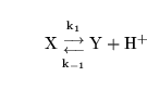 |
(36) |
the halftime to reach equilibrium under conditions of constant pH is:
![\begin{displaymath}
t_{1/2} = \frac{\ln(2)}{\ensuremath{\mathrm{k_1 + k_{-1}[H^+]}}}
\end{displaymath}](img109.png) |
(37) |
giving
![\begin{displaymath}
\ensuremath{\mathrm{k_1}}= \frac{\ln(2)}{t_{1/2}(\ensuremath...
...}}}= \frac{\ln(2)}{t_{1/2}(\ensuremath{\mathrm{Keq + [H^+]}})}
\end{displaymath}](img110.png) |
(38) |
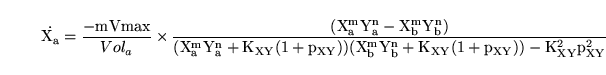
Carrier mediated transport
Carrier mediated transport can be modelled using the methodology described in Section 2.4.1 of (3). If
 exists in two compartments
  and
and  with concentrations
 and
, then the theoretical reaction scheme is:
and
, then the theoretical reaction scheme is:
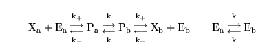 |
(39) |
where
 is the carrier and
 is the complex of carrier and
. The steady state assumption leads to evolution of the form:
is the complex of carrier and
. The steady state assumption leads to evolution of the form:
![\begin{displaymath}
\dot [\ensuremath{\mathrm{X_a}}] = \frac{-\ensuremath{\mathr...
...rm{[X_b] + K_X(1 + p_X)}}) - \ensuremath{\mathrm{K_X^2p_X^2}}}
\end{displaymath}](img118.png) |
(40) |
where
 is a constant reflecting the equilibrium in the binding of
to the carrier, and
is a constant reflecting the equilibrium in the binding of
to the carrier, and
 is the ratio of the rates of conversion between the different states of the carrier, and the rate of binding of
to the carrier.
is the ratio of the rates of conversion between the different states of the carrier, and the rate of binding of
to the carrier.
 is not strictly a maximum rate - the maximum rate of transport for a given
![$[\ensuremath{\mathrm{X_b}}]$](img122.png) is:
is:
![\begin{displaymath}
\frac{-\ensuremath{\mathrm{Vmax}}}{Vol_a(\ensuremath{\mathrm{[X_b] + K_X(1 + p_X)}})}
\end{displaymath}](img123.png) |
(41) |
It is usually
 values which are quoted in textbooks. If we assume that
 reprents the concentration of
across the membrane at which we have half-maximal transport, when concentration on the other side is zero, we can calculate that:
reprents the concentration of
across the membrane at which we have half-maximal transport, when concentration on the other side is zero, we can calculate that:
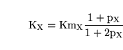 |
(42) |
In the case of symport, we again follow (3) and assume that all intermediate steps can be ignored. Thus if substrates X and Y are transported together we assume the reaction scheme:
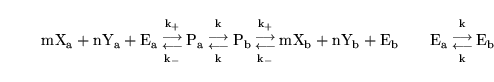 |
(43) |
giving rise to dynamics of the form:
 |
(44) |
Next: Metabolic rates and accounting
Up: All model parameters
Previous: Basics
Murad Banaji
2004-07-08
![$\displaystyle -\left(\ensuremath{\mathrm{k_1}}\sum_{i=1}^{z_1}\left[ \ensuremat...
...{\partial \mathcal{G}_2}{\partial b_i}\right]\right)\alpha_k \quad \mbox{any k}$](img85.png)
![$\displaystyle -\left(\ensuremath{\mathrm{k_1}}\sum_{i=1}^{z_1}\left[ \ensuremat...
...c{\partial \mathcal{G}_2}{\partial b_i}\right]\right)\beta_k \quad \mbox{any k}$](img87.png)