Subsections

• Consistency and model constraints

Basics

The basic philosophy of parameter setting is as follows:

• Where parameters are easily available in the literature we use these
• We attempt to use parameters which we have clear intuitive meaning and which we have some hope of finding in the literature to estimate values of parameters which are model dependent.

There are many problems inherent in attempting to estimate parameters in such a large model. However we have made the following empirical observation: As the model has grown and become more realistic, there are fewer and fewer parameters to whose precise values the model is very sensitive. Although this cannot in any sense be phrased as a ``theorem'' it does give some hope about the whole process of constructing biological models. Presumably it reflects the fact that biological systems have evolved to be robust.

Underlying much of our parameter setting is the assumption that at ``normal'' fixed parameter values, the model should tend to a steady state. Although there are parameter values where the model shows periodic or even chaotic behaviour, so far all iterations of the model show the presumed steady state behaviour at normal values.

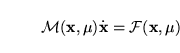
Starting with this assumption, the process of estimating parameters proceeds as follows. The model is defined by a set of differential and algebraic equations assumed to be time independent:

$$\mathcal{M}({\mathbf x}, \mu)\dot{\mathbf x} = \mathcal{F}({\mathbf x}, \mu)$$ (1)

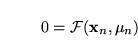
Here ${\mathbf x}$ describes the set of all model variables, $\mathcal{M}$ is the ``mass matrix'' which is in general singular (1), $\mu$ represents the parameter set, and a dot over a variable represents differentiation with respect to time. Assuming a steady state means assuming that there exist values of the variables $\mathbf{x = x_n}$ for ``normal'' parameters $\mu = \mu_n$, such that there is a solution to the equation:

$$0 = \mathcal{F}({\mathbf x_n}, \mu_n)$$ (2)

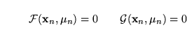
Apart from this equation which depends only on the model structure and the functional form of $\mathcal{F}$, there are in general further constraints on the normal model behaviour. An example of such a constraint is to fix for example the normal metabolic rate for oxygen. Let all such constraints comprise a new set of equations, 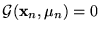$\mathcal{G}({\mathbf x_n}, \mu_n) = 0$. Then we have the combined system:

$$\mathcal{F}({\mathbf x_n}, \mu_n) = 0 \qquad \mathcal{G}({\mathbf x_n}, \mu_n) = 0$$ (3)

We assume that this system can be reduced to $N$ non-degenerate equations. We can then choose $N$ quantities from among $\{\mathbf x_n\}$, $\{\mu_n\}$ to solve for.

This notion of solving for some of the parameter values in this way is not frequently encountered in biological modelling, but is central to our approach. Given the size of the system, it is unrealistic to hope to solve equation 3 all at once. However we can use this principle and the fact that the equations have some structure (a skew product structure to be precise) to help in the task.

Consistency and model constraints

The main difficulties with the above approach are the tendency to get

• An overdetermined system (too many equations for too few variables, or the equations have no solutions)
• An underdetermined system (not enough equations to determine all the quantities left as unknowns)
• Computational difficulties in actually solving the equations.

To illustrate the first, consider the following mass-action reaction:

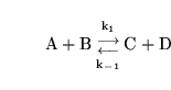$$\ensuremath{\mathrm{A + B {{\ensuremath{\mathrm{k_1}}\atop{\... ... {{\longleftarrow}\atop{\ensuremath{\mathrm{k_{-1}}}}}} C + D}}$$ (4)

Suppose we have values for the steady state concentrations of $\ensuremath{\mathrm{A}}$, $\ensuremath{\mathrm{B}}$, $\ensuremath{\mathrm{C}}$ and $\ensuremath{\mathrm{D}}$ - $\ensuremath{\mathrm{[A]_n}}$, $\ensuremath{\mathrm{[B]_n}}$, $\ensuremath{\mathrm{[C]_n}}$ and $\ensuremath{\mathrm{[D]_n}}$. Suppose we also know the ``cerebral metabolic rate of $\ensuremath{\mathrm{A}}$'' - say that at steady state there is net conversion of $2$ $\ensuremath{\mathrm{\mu M/mL/s}}$ of $\ensuremath{\mathrm{A}}$ into $\ensuremath{\mathrm{C}}$ and $\ensuremath{\mathrm{D}}$. Then we must have that:

$$\ensuremath{\mathrm{k_1[A]_n[B]_n - k_{-1}[C]_n[D]_n = 2}}$$ (5)

In this situation if we find values in the literature for $\ensuremath{\mathrm{k_1}}$ and $\ensuremath{\mathrm{k_{-1}}}$, we might not be able to plug these in without violating our condition about the steady state use of $\ensuremath{\mathrm{A}}$. The reason might be that we are omitting some other processes which actually contribute to the steady state consumption of $\ensuremath{\mathrm{A}}$. In such a situation, we have to decide whether to use the given rate constants or to ensure that equation 5 is fulfilled.

As a particular example from the current model, we assume that the only active process which pumps potassium ions into cells and sodium out is via $\ensuremath{\mathrm{Na^+,K^+}}$-ATPase, and involving 3 for 2 exchange of sodium for potassium. This means however that for the model to be at steady state, the normal rates of sodium influx into cells and potassium efflux from cells (due to leakage, and neural firing) must also be in a three to two ratio. Parameters in our caricature of neural firing must be set in such a way as to ensure this condition.

The second difficulty - an underdetermined system - needs no example. As every biological modeller knows, it can be hard to obtain estimates for parameters. Much of what follows is concerned with estimating parameters from heuristic arguments, or from quantities which are more likely to have been measured.

The final difficulty - computational problems with solving the actual equations - has not been entirely resolved. In theory, if we have a particular variable $y$ and use the putative steady state value of this variable $y_n$ to estimate other parameters, when the model is actually run, the value of $y$ should converge to $y_n$. But because we do not actually solve system 3 all at once, and because there are various points where estimates have to be made, this isn't always the case. For example, we estimate the total diffusion rate of $\ensuremath{\mathrm{CO_2}}$ across the blood brain barrier from estimates of the normal concentration of $\ensuremath{\mathrm{CO_2}}$ on either side of the barrier, and the normal rate of production of $\ensuremath{\mathrm{CO_2}}$. But these last quantities depend in complicated ways on the rest of the model, and on other estimates, and we cannot necessarily get the values exactly right. Currently, we tolerate a certain amount of error in these situations, although in theory it is possible to develop schemes which ensure model consistency.