Next: A list of model
Up: All model parameters
Previous: Particular calculations: biochemistry
Subsections
Total potassium channel conductivity of a given VSM segment
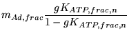
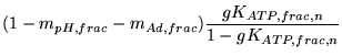
The total potassium channel conductivity of a segment is the sum of the conductivities of different kinds of channels. We can first calculate the total conductivity from an estimate of the normal membrane potential in a segment and some idea of the ionic species of interest. If we assume that the primary ions of interest to us in VSM are
 ,
,
 and
and
 we have (see p51 of (8)):
 |
(88) |
Note that this linear model has been found not to adequately describe some membranes (9). We allow for the possibility that the full Goldman-Hodgkin-Katz equation (3) might replace the linear model in revisions of our model.
If we wish to emphasise that we are only ever interested in the ratios of the conductivities to sodium and chlorine to that of potassium, we can rewrite this equation:
 |
(89) |
From this we get the normal value of gK in a given segment:
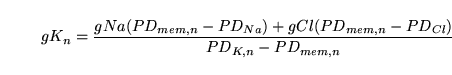 |
(90) |
where we assume that the other quantities can be measured or estimated.
The next task is to estimate the contributions from the different kinds of channel to this basal conductivity. Since:
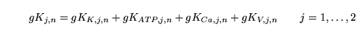 |
(91) |
These estimates are hard to obtain from the literature, so there is some guesswork involved. It is an interesting exercise to see how sensitive the model is to different choices.
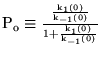
Consider a two-state ion channel which is activated by stimuli X and inhibited by stimuli Y, leading at steady state to an open probability of the form:
![\begin{displaymath}
\ensuremath{\mathrm{\frac{[Ch_o]}{Ch_{tot}} = \frac{k_1(X)}{k_{-1}(Y) + k_1(X)}}}\end{displaymath}](img285.png) |
(92) |
where
![$[\ensuremath{\mathrm{Ch_o}}]$](img286.png) is the number of open ion channels,
is the number of open ion channels,
 is the total number of ion channels and
 and
and
 are functions which represent the way in which the stimuli affect the channel. The above equation can be rewritten as:
![\begin{displaymath}
\ensuremath{\mathrm{\frac{[Ch_o]}{Ch_{tot}} = \frac{\frac{k_1(X)}{k_{-1}(Y)}}{1 + \frac{k_1(X)}{k_{-1}(Y)}}}}\end{displaymath}](img288.png) |
(93) |
In general we will have chosen some general form for
and
- say affine (
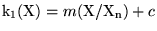 ) or exponential (
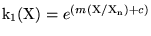 ). Since we are only interested in the quotient
 , we can stipulate that at normal values of Y, i.e.
 , we have
 . A quantity we can sometimes find/estimate from the literature is the normal proportion of open channels:
![\begin{displaymath}
\ensuremath{\mathrm{\frac{[Ch_o]}{Ch_{tot}}(X_n, Y_n) \equiv P_n = \frac{k_1(X_n)}{1 + k_1(X_n)}}}\end{displaymath}](img294.png) |
(94) |
It is also possible that we might find or be able to estimate quantities such as
 . Such estimates can be used to calculate the values of parameters in the functions
and
.
. Such estimates can be used to calculate the values of parameters in the functions
and
.
Normal potassium channel conductivities
We now apply these ideas to each of the different types of potassium channels. Where each VSM segment is treated identically to simplify the notation we drop the subscript indicating a particular segment.
For inward rectifier potassium channels we have:
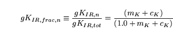 |
(95) |
Assuming that we have estimates for
 and
and  we can immediately calculate
  . We also see that:
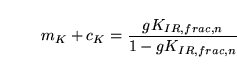 |
(96) |
 represents the background level of channel opening in the absence of the stimulus (potassium ions in the extracellular space). Define
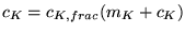 . We then have:
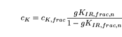 |
(97) |
and
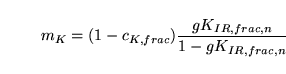 |
(98) |
We now treat ATP sensitive channels. We have that:
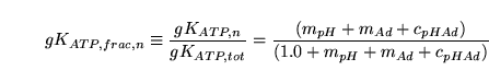 |
(99) |
Again we can immediately calculate  . And we have that
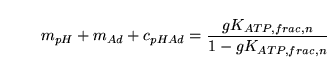 |
(100) |
Defining  by
by
 , and similarly for
  , we have:
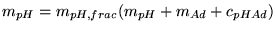
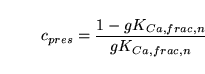
We now treat calcium-sensitive channels. We have that:
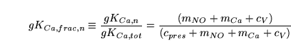 |
(104) |
Again we can immediately calculate  . From the arguments above we can set:
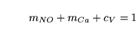 |
(105) |
We then also have:
 |
(106) |
We have for the conductivity of voltage gated potassium channels :
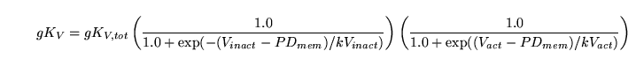 |
(107) |
For these channels the situation is somewhat different from the others since we have reasonable estimates for the four parameters involved. We can thus calculate  from:
from:
 |
(108) |
Calcium channels in VSM
First we note that the normal equilibrium potential for calcium in the  th VSM segment,
  , is simply calculated from the equation:
![\begin{displaymath}
PD_{Ca, j, n} = \frac{C_{el}}{2}\ln\left(\frac{\ensuremath{\mathrm{[Ca_{e}]_n}}}{\ensuremath{\mathrm{[Ca_{i, j}]_n}}}\right)
\end{displaymath}](img326.png) |
(109) |
where  is a lumped constant equal to RT/F where R is the gas constant, T is body temperature in Kelvin and F is the Faraday constant, and
![$\ensuremath{\mathrm{[Ca_{e}]_n}}$](img328.png) , the extracellular concentration of calcium, is taken to be a constant.
, the extracellular concentration of calcium, is taken to be a constant.
Now we remind ourselves from section 4.4 that
 , the normal rate of inflow of calcium into the th VSM segment can be determined from knowledge of the normal calcium dynamics in the segment. But the parameters
are closely related to the normal conductivities of these channels, since:
, the normal rate of inflow of calcium into the th VSM segment can be determined from knowledge of the normal calcium dynamics in the segment. But the parameters
are closely related to the normal conductivities of these channels, since:
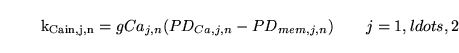 |
(110) |
This equation can be used to determine 
Currently the only stimulus which affects the conductivity of calcium channels is the membrane potential. Further, inactivation is assumed not to be important at physiological membrane potentials. So we get:
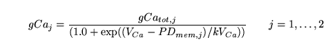 |
(111) |
As with voltage gated potassium channels, since the parameters are available in the literature we calculate  from:
from:
 |
(112) |
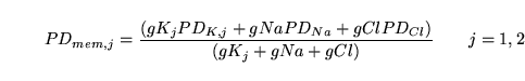
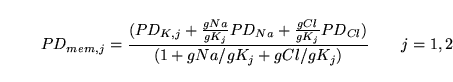
Extracellular potassium is known to have both vasodilatory and vasoconstrictory effects on blood vessels depending on its concentration (chapter 9 of (8) for example). The vasodilatory effect at low potassium concentrations is assumed in the model to occur primarily via the activation of inward rectifier potassium channels. The vasoconstrictory effect on the other hand occurs by alteration of the equilibrium potential for potassium, a major determinant of the resting membrane potential.
In order to check whether the model is able to reproduce this behaviour we explore the response of the membrane potential to extracellular potassium in the model. We have in the model that the total potassium channel conductivity in a given section is:
![\begin{displaymath}
gK_{tot} = gK_o + gK_{IR} = gK_o + gK_{IR, tot}\frac{\left(m...
...m{\frac{[K^+_{ec}]}{[K^+_{ec}]_n}}}\right)^{n_K} + c_K\right)}
\end{displaymath}](img334.png) |
(113) |
where  represents the conductivity of all potassium channels other than the inward rectifier channels.
We also know that the equilibrium potential for potassium is:
![\begin{displaymath}
PD_K = C_{el}\ln\left(\frac{[\ensuremath{\mathrm{K^+_{ec}}}]}{[\ensuremath{\mathrm{K^+_{ic}}}]}\right)
\end{displaymath}](img336.png) |
(114) |
where is defined in Section 5.4 and
 refers to the concentration of potassium ions inside the muscle cells which is for simplicity taken to be constant. We then have for the membrane potential from equation 89:
![\begin{displaymath}
PD_{mem} = \frac{C_{el}\ln\left(\frac{[\ensuremath{\mathrm{K...
...[K^+_{ec}]_n}}}\right)^{n_K} + c_K\right)}\right) + gNa + gCl}
\end{displaymath}](img338.png) |
(115) |
Assuming that is constant and plotting  as a function of
![$[\ensuremath{\mathrm{K^+_{ec}}}]$](img340.png) we see that at typical parameter values we do indeed see the biphasic response observed, as long as
we see that at typical parameter values we do indeed see the biphasic response observed, as long as  is greater than 1 and the inward rectifier channels provide a significant proportion of resting potassium channel conductivity. Thus there is a range of values of extracellular potassium where increasing the concentration decreases the membrane potential, implying that the activation of potassium channels is the dominant effect. Because of the assumption that intracellular potassium remains constant, at very low extracellular potassium concentrations, the equilibrium potential and hence the membrane potential becomes very large and negative, but this behaviour is unphysical, implying a large potassium gradient.
Next: A list of model
Up: All model parameters
Previous: Particular calculations: biochemistry
Murad Banaji
2004-07-08