


Up: Index of documentation
Modelling chemical reactions, transport processes and ion channels
We summarise how chemistry and transport processes can be translated into the language of mathematics. If, given a process of interest, we have a limited set of conventions for how to extract terms in equations from this process, then the task of model description is greatly simplified. Furthermore the computational task of model construction is greatly simplified.
Much of what we present below is standard and can be found in textbooks on mathematical physiology such as (1). However some of it is non-standard.
We need a few notational conventions. Where a chemical X can exist in several compartments, we represent this with subscripts. For example
Xa
refers to the concentration of X in some compartment A, and throughout the documentation,
Xc
,
Xec
,
Xcyt
and
Xim
refer to X in the capillaries, extracellular space, intracellular (but extramitochondrial) space and mitochondrial spaces respectively. Sometimes, when it is clear from context which compartment a given chemical resides in, the subscripts are omitted for conciseness. The concentration of X is represented as usual by [X]. Ellipses ( ...
) in a differential equation refer to the existence of other terms which we omit. So for example when we explain how a process contributes a term to a differential equation for a variable, we usually take it as understood that other processes might contribute other terms to the same differential equation.
The first type of reaction we consider is the best known and most basic. Mass action reactions can be reversible or irreversible, and are described by one or two rate constants. Irreversible reactions are a special case of reversible reactions with one rate constant set to zero, and so we do not have to treat them separately. Consider the reaction:
 |
(1) |
This equation contributes a term to each O.D.E. describing the evolution of each of the chemicals involved in it. For example it gives rise to the dynamics
![\begin{displaymath}
\ensuremath{\mathrm{\dot {[A]}}} = -2\ensuremath{\mathrm{k_{...
...}}\ensuremath{\mathrm{[B]}} \ensuremath{\mathrm{[C]}}\cdots
\end{displaymath}](img4.png) |
(2) |
for the evolution of A. Of course A may be involved in other processes in which case the differential equation for A will contain other terms.
We do not only use mass action reactions in situations where this is known to be the best description of the reaction. Rather they are treated as the ``default'' - the most basic kind of reaction to be used where the alternatives are too complicated or poorly understood too.
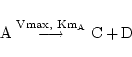
Perhaps it would be ideal to represent all reactions via complete mass action schemes. However a lack of data on the detailed mechanisms of reactions, and on values of rate constants means that it is necessary to introduce other approximations. The first such is the Michaelis-Menten formalism (see (1) for the details). Michaelis-Menten reactions are considered to be one-way, and a reversible reaction is represented as two irreversible ones. Consider for example:
 |
(3) |
This generates terms in ODEs:
![\begin{displaymath}
\ensuremath{\mathrm{\dot {[A]} = -\frac{Vmax [A]}{Km_A + [A]} \cdots}}
\end{displaymath}](img7.png) |
(4) |
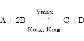
When there is more than one substrate, each has its own Km value. E.g.
 |
(5) |
which leads to terms such as:
![$\displaystyle \dot{{[\mathrm{B}]}}$](img10.png) = - 2 = - 2![$\displaystyle {\frac{{\mathrm{Vmax[A][B]^2}}}{{(\mathrm{Km_A + [A]})(\mathrm{Km_B^2 + [B]^2})}}}$](img11.png) = - 2 = - 2![$\displaystyle {\frac{{\mathrm{Vmax}}}{{\mathrm{(1 + Km_A/[A])(1 + (Km_B/[B])^2)}}}}$](img12.png) = - 2 = - 2![$\displaystyle {\frac{{\mathrm{Vmax}}}{{\mathrm{(1 + Km_A/[A] + (Km_B/[B])^2 + Km_AKm_B^2/([A][B]^2))}}}}$](img13.png) ... ...
|
(6) |
Based on the final form above, a slightly more flexible expression is:
![\begin{displaymath}
\ensuremath{\mathrm{\dot {[B]} = -2\frac{Vmax}{(1 + Km_A/[A] + (Km_B/[B])^2 + Km_{AB}/([A][B]^2))}\cdots}}
\end{displaymath}](img14.png) |
(7) |
where
KmAB
is a new parameter. Of course this requires estimation of more parameters.
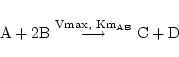
Occasionally we might have a Michaelis-Menten reaction with more than one substrate, but assume that they combine before coming into contact with the enzyme. We then write the chemical equation:
 |
(8) |
which leads to terms like:
![\begin{displaymath}
\ensuremath{\mathrm{\dot {[B]} = -2\frac{Vmax[A][B]^2}{(Km_{AB} + [A][B]^2)} \cdots}}
\end{displaymath}](img17.png) |
(9) |
and so on.
It is worth noting that in the current version of the model we sometimes treat reversible enzyme-mediated reactions as though they were simple mass action reactions. Sometimes this can be justified on the basis that the reaction is normally at equilibrium in vivo and hence we are not very interested in its transient behaviour. On the other hand, sometimes this simplification is made simply for convenience (i.e. largely due to the difficulty in finding reliable Km values for all the substrates and products) and cannot be justified on any physiological basis.
We allow for the possibility that other substances can inhibit or activate enzymes competitively or noncompetitively by altering the Km and Vmax values (see the discussion in Chapter 6 of (2)).
Generalised reactions (GR)
Often we model multiple/complex processes as simpler ones. By way of example consider the two reactions:
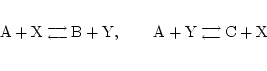 |
(10) |
These could be seen as one reaction:
 |
(11) |
However we would in general get incorrect dynamics if we assumed that this was a normal mass action reaction.
In such situations where we are ignoring the detailed mechanism of the reaction, the only thing that we can say is that the stoichiometries must be correctly preserved. In the example above, this means that there must be some function
 ([A],[B],[C])
such that
([A],[B],[C])
such that
![\begin{displaymath}
\ensuremath{\mathrm{\dot {[A]}}} = -2\mathcal{F}(\ensuremath...
...C]}}} = \mathcal{F}(\ensuremath{\mathrm{[A], [B], [C]}})\cdots
\end{displaymath}](img25.png) |
(12) |
We call such a reaction, which does not a priori give rise to a particular form for
a ``generalised reaction''. We often apply the notion of generalised reactions in situations such as the above where we combine several reactions into one, or use empirically derived functional forms.1 In general if we have a generalised reaction:
 |
(13) |
we must state the rate term associated with this reaction.
We refer the reader to Chapter 2 of (3) for a more complete discussion.
Sometimes we have cause to treat a process as zeroth order. For example a reaction of the form:
 |
(14) |
implies the production of A at a rate independent of any chemical concentration. It leads to dynamics of the form:
![\begin{displaymath}
\ensuremath{\mathrm{\dot {[A]} = k_1 \cdots}}
\end{displaymath}](img31.png) |
(15) |
In such situations the implicit assumption is of a source of A from which A is being extracted, with the source concentration of A not affecting the extraction of A. This could be either because the concentration in the source is held fixed (by processes external to the model) or because extraction is rate-limited by chemical/transport process within the normal limits of variation of A in the source.
While we allow zeroth order production, we avoid having processes which involve zeroth order use of a chemical - i.e. use of a chemical at a rate independent of its concentration. If the chemical is being modelled, then this would be a recipe for getting unphysical negative concentrations.
Transport of substances between different compartments
We make some general remarks about transfer of substances between different compartments, or reactions which involve substances on different sides of a membrane (
Na+ - K+
-co-transport, malate-aspartate shuttle, etc.) Indeed if we have a substance X which lives in two compartments a
and b
with volumes Vola
and Volb
, then we can treat passive diffusion between the compartments as a chemical reaction:
 |
(16) |
However the rate constant has a somewhat different meaning (and different units) from normal, and would now represent the rate of transport of absolute quantities of X. If for example [X] was measured in
 , we would expect
kX
to have units not of
s-1
, but of ml/s. So for example, for the differential equations for
[Xa]
and
[Xb]
we would derive the following terms:
, we would expect
kX
to have units not of
s-1
, but of ml/s. So for example, for the differential equations for
[Xa]
and
[Xb]
we would derive the following terms:
![\begin{displaymath}
\ensuremath{\mathrm{\dot{[X_a]}}} = -\frac{\ensuremath{\math...
...thrm{k_x}}}{Vol_b}(\ensuremath{\mathrm{[X_a] - [X_b]}}) \cdots
\end{displaymath}](img36.png) |
(17) |
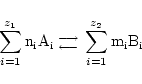
Carrier mediated transport can be modelled as in Section 2.4.1 of (1). The theoretical reaction scheme is:
 |
(18) |
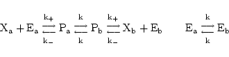
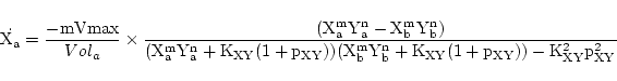
where E is the carrier and P is the complex of carrier and X. The steady state assumption leads to evolution of the form:
 |
(19) |
where
KX
is a constant reflecting the equilibrium in the binding of X to the carrier, and
pX
is the ratio of the rates of conversion between the different states of the carrier, and the rate of binding of X to the carrier. A little algebra then allows us to relate the rate constants Vmax,
KX
and
pX
to those traditionally given in text books.
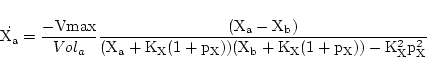
In the case of symport, we again follow (1) and assume that all intermediate steps can be ignored. Thus if substrates X and Y are transported together we assume the reaction:
 |
(20) |
giving rise to dynamics of the form:
 |
(21) |
We represent such a reaction as:
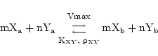 |
(22) |
Detailed models of active transport require some insight into the mechanisms involved - see for example Section 2.5 of (1) and give rise to complicated functional forms for the relevant reaction rates, with the consequent estimation of a number of parameters. Currently we ignore such complications, although this is something that might be changed in model updates. Instead we simply treat the reactions as Michaelis-Menten reactions involving substances on different sides of the barrier. Essentially this ignores the multiple states that the carrier molecule can exist in, and assumes that the rate of reaction is limited by the rate of combination of the chemicals to be transported (and ATP or any other substrate which provides energy for the transport) with the carrier. Thus if we represent the reaction as:
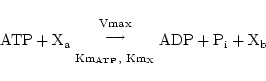 |
(23) |
we imply the extraction of rate terms of the form:
![\begin{displaymath}
\ensuremath{\mathrm{\dot {[X_a]}}} = -\frac{\ensuremath{\mat...
...\ensuremath{\mathrm{(Km_X + [X_a])(Km_{ATP} + [ATP])}}} \cdots
\end{displaymath}](img54.png) |
(24) |
If we want to ignore the use of ATP in such a process we might simply write a reaction as:
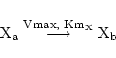 |
(25) |
implying dynamics of the form:
![\begin{displaymath}
\ensuremath{\mathrm{\dot {[X_a]} = -\frac{Vmax[X_a]}{Vol_a(Km_X + [X_a])} \cdots}}
\end{displaymath}](img58.png) |
(26) |
Sometimes transport across a barrier can be by a mixture of active and passive means. Another possibility is transport linked to the transport of a species which we do not model. Or quite simply information on the precise mechanisms of transport might be unavailable, although the steady state values can be found. In such cases we usually assume the reaction:
 |
(27) |
where this time the two rate constants need not be equal. We would then for example have the term:
![\begin{displaymath}
\ensuremath{\mathrm{\dot{[X_a]}}} = -\frac{1}{Vol_a}\left(\ensuremath{\mathrm{k_x[X_a] - k_{nx}[X_b]}}\right) \cdots
\end{displaymath}](img61.png) |
(28) |
for the evolution of
Xa
, with a similar term for
Xb
.
Convective transport
There are convective processes of various kinds to be modelled. Convection of a chemical X through a compartment b
is simplified if we can assume either that there is only one convection process (i.e. only inflow or outflow) or that the sites of inflow and outflow within a given compartment contain chemicals at the same concentration (rapid mixing within the compartment). Assuming that any rate of change of the compartment's volume is negligible in comparison to the rate of bulk flow, inflow and outflow rates (of the solute) must be equal - say q
, and then the transport in and out of
Xb
is given by:
![\begin{displaymath}
\dot \ensuremath{\mathrm{[X_b]}} = \frac{q}{Vol_b}\ensuremath{\mathrm{([X_a] - [X_b])}} \cdots
\end{displaymath}](img62.png) |
(29) |
where
[Xa]
is the concentration of X flowing in. If say, there is no inflow process, this becomes:
![\begin{displaymath}
\dot \ensuremath{\mathrm{[X_b]}} = -\frac{q}{Vol_b}\ensuremath{\mathrm{([X_b])}} \cdots
\end{displaymath}](img63.png) |
(30) |
(Obviously in this case
[Xb]
tends to zero unless there is some other process producing X in b
.)
When, as in the capillary compartment, we cannot assume that there are no chemical gradients, an alternative methodology must be employed. In this case we use the form:
![\begin{displaymath}
\dot \ensuremath{\mathrm{[X_b]}} = \frac{2q}{Vol_b}\ensuremath{\mathrm{([X_a] - [X_b])}} \cdots
\end{displaymath}](img64.png) |
(31) |
The term 2q
arises from the crude discretisation of a convective P.D.E.
A general paradigm for treating stimulus induced changes in ion channel conductance
Ion channels are essentially treated as chemical objects in our model. Here we sketch the way we treat ion channels and warn the reader that this is very simplistic and currently ignores the considerably more complex modelling possibilities (see for example (1)).
Basically, we treat ion channels as two state objects - i.e. they can be either open or closed. Given a channel Ch, we label these two states
Cho
and
Chc
respectively. Let us assume that the interconversion of
Cho
and
Chc
is governed by rate constants
k1
and
k-1
.
By way of example, we assume that some stimulus or combination of stimuli X activates the channel - i.e. increases the rate of channel opening, and on the other hand some other stimulus Y, inhibits the channel (which we can represent as increasing the rate of channel closure):
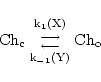 |
(32) |
We get at equilibrium:
![\begin{displaymath}
\ensuremath{\mathrm{\frac{[Ch_o]}{[Ch_c]} = \frac{k_1(X)}{k_{-1}(Y)}}}
\end{displaymath}](img69.png) |
(33) |
Defining the total concentration of channels
[Cho] + [Chc]  Chtot
, we get:
Chtot
, we get:
![\begin{displaymath}
\ensuremath{\mathrm{\frac{[Ch_o]}{Ch_{tot}} = \frac{k_1(X)}{k_{-1}(Y) + k_1(X)}}}
\end{displaymath}](img73.png) |
(34) |
The left hand side of this equation is the proportion of open channels. Clearly the right hand side can only vary between 0 and 1 whatever the functional forms chosen.
The assumption that channels are two state objects ignores the fact that many channels can be inactivated, and that the inactivation rate itself might depend on the stimuli. In order to introduce some flexibility we allow for this possibility by assuming that there might be a further inactivation function
f (X, Y)
multiplying the right hand side in equation 34 to give:
![\begin{displaymath}
\ensuremath{\mathrm{\frac{[Ch_o]}{Ch_{tot}}}} = f(\ensuremat...
...rm{Y}})\ensuremath{\mathrm{\frac{k_1(X)}{k_{-1}(Y) + k_1(X)}}}
\end{displaymath}](img74.png) |
(35) |
The next step is to choose appropriate functional forms for
k1
and
k-1
. One choice might be affine, i.e. of the form
k1(X) = m(X/Xn) + c
, etc. Here
Xn
represents the baseline levels of X, c
represents the residual rate of opening in the absence of X, and m
represents just how large the effect of a unit increase in
X/Xn
is on the rate of opening. (We often normalise the value of a variable with respect to some typical value for convenience.) Note that X need not represent a chemical concentration, but could represent a voltage, or a pressure difference for example.
Of course an affine function is not the only possibility. Other possibilities are higher order polynomials say
k1 = m(X/Xn)n + c
(leaving out the lower order terms implies an assumption of a particular mechanism, say that n
molecules of X must bind to a channel to open it) or exponential functions, say
k1 = e(m(X/Xn)+c)
, which might perhaps be appropriate within certain limits for a quantity such as membrane potential which can take both positive and negative values.
The biological motivations for the forms chosen for
k1(X)
and
k-1(X)
are not always obvious or simple. On the occasions where the stimulus is a chemical one, then there can be justifications for the form, based on assumptions about the number of molecules of X which must bind to
Chc
in order to open it. On the other hand when X is a biophysical stimulus such as pressure or membrane potential (possibly with a very complex transduction mechanism) attempts to use experimental data to find a functional form are probably wisest.
Currently we always assume that gating is a fast process and hence that we are only interested in the equilibrium behaviour of the channel. This allows us to arbitrarily set either
k1(X)
or
k-1(Y)
to 1 at normal values of the stimuli. However we are aware that this assumption may need to be revised. Note that if we choose
k-1(Y) = 1
, then
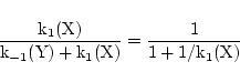 |
(36) |
a form we often use.
- 1
-
J. Keener, J. Sneyd, Mathematical Physiology, Vol. 8 of Interdisciplinary
Applied Mathematics, Springer, 1998.
- 2
-
N. Bhagavan, Medical Biochemistry, Harcourt/Academic Press, 2002.
- 3
-
R. Heinrich, S. Schuster, The regulation of cellular systems, Chapman and Hall,
1996.
Up: Index of documentation
Murad Banaji
2004-07-08